Move Pivot Table in Excel
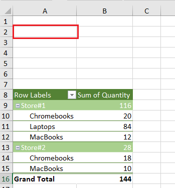
As you can see in the image below, the Pivot Table is starting from Row 8 (Cell A8) with unnecessary empty Rows at the top. This issue can be easily corrected by moving the Pivot Table to Cell A2.
Similarly, you may come across the need to move Pivot Table to a new Worksheet within the same Workbook or to New Worksheet in another Workbook. All these tasks can be easily achieved by making use of the Move PivotTable command as available in Microsoft Excel.
1. Move Pivot Table Within the Same Worksheet
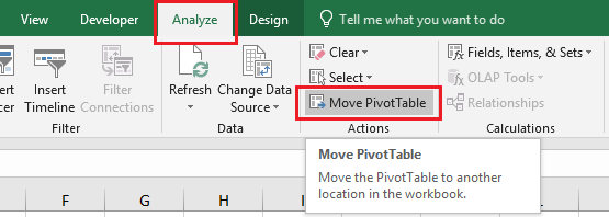
Follow the steps below to move Pivot Table to another area on the same worksheet 1.1. Click anywhere on the Pivot Table. 1.2. Next, click on the Analyze tab located in the top menu bar and click on Move PivotTable option.
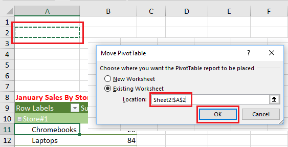
1.3. On the Move PivotTable dialogue box, click in the Location box and then click on the New location where you want to move the Pivot Table and click on OK.
In the above example, we have clicked in Cell A2 in order to move the Pivot Table to this location.
2. Move Pivot Table to New or Another Worksheet
Most of the time, you may come across the need to move Pivot Table to a New Worksheet. This way the Pivot Table will be housed in its own separate Worksheet. 2.1. Click anywhere on the Pivot Table. 2.2. Next, click on the Analyze tab located in the top menu bar and then click on Move PivotTable option.
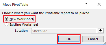
Note: Move PivotTable option may also be located under PivotTable Options Tab. 2.3. On the Move PivotTable dialogue box, select New Worksheet option and click on OK.
Excel will automatically open a new worksheet and the Pivot Table will be moved to the New Worksheet.
3. Move Pivot Table to Another Workbook
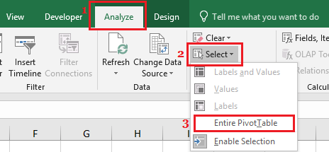
There is really no option in Excel to move Pivot Table to another workbook. However, it is possible to copy the Pivot Table and paste it in another workbook. 3.1. Click anywhere on the Pivot Table. 3.2. Next, click on the Analyze tab located in top menu bar > click on Select and then click on Entire PivotTable option in the drop-down menu.
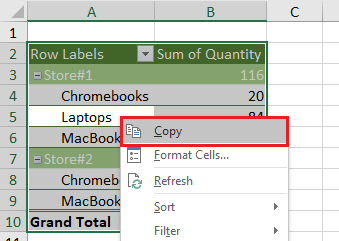
Note: You may find Move PivotTable option located under PivotTable Options Tab. 3.3. Once the Pivot Table is selected, right-click on it and click on the Copy option.
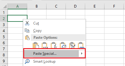
3.4. Now navigate to the other Workbook > right-click on the cell at which you want the Pivot Table to start and then click on Paste Special option in the menu that appears.
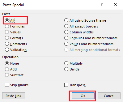
3.5. On the Paste Special screen, make sure that “All” option is selected and click on OK.
You will immediately see the Pivot Table being pasted in the New Workbook. The pasted Pivot Table should retain most of its formatting and you may only be required to adjust the column widths.
How to Change Pivot Table Data Source and Range How to Add or Remove Subtotals in Pivot Table

